Author Archives: Christopher Kam

In this post, I consider the proportionality of the Alternative Vote (AV), that is, the degree to which AV produces a 1:1 ratio between parties’ vote shares and their seat shares. (AV is the electoral system that is purportedly the Liberal’s favoured alternative to replace Canada’s first-past-the-post electoral system (FPTP).)

By using data from Australian federal elections as well as state elections in Australia’s five mainland states, we can see how AV tends to perform in six different polities.* Moreover, because these jurisdictions all employed FPTP at some point in time, we can also consider whether the shift to AV altered the votes-seats proportionality of Australian elections. This should give us some idea of what to expect should Canada adopt AV.

A priori, we should not expect AV to be any more or less proportional than FPTP. The reason is that both system tend to employ single-member districts. The number of seats per district—what political scientists call the district magnitude—constrains the proportionality of an electoral system quite independently of the formula that is used to translate votes into seats. The higher the district magnitude, the more closely the division of seats among parties can approximate the distribution of vote shares among parties. This improves the votes-seats proportionality of the electoral system. Conversely, votes-seats proportionality that is achievable declines as the district magnitude moves to 1.

Understand that the impact of district magnitude on votes-seats proportionality operates at the district-level. It’s quite possible for an electoral system based on single-member districts to be proportional in aggregate even as it is highly disproportional in every district. Imagine a polity with three parties (A, B, C) competing in FPTP elections in three single-member districts (1,2 3). Assume that party A wins 34% of the vote in district 1 versus 33% for parties B and C, respectively. Similarly, B wins district 2, and C wins district 3, on identical divisions of the vote, that is, 34% – 33% – 33%. The result is a high degree of disproportionality within each district (the party winning 34% of the vote obtaining 100% of the district’s seats) but perfect proportionality in the aggregate, each party winning 1/3 of the seats on 1/3 of the vote.

Of course, district-level disproportionality need not (and often does not) cancel out across districts; it may well be compounded. Indeed, in the past governing parties would intentionally gerrymander and malapportion districts to ensure that disproportionality compounded across districts: district boundaries were drawn to ensure that the government won the vast majority of seats by razor-thin margins whilst the opposition’s votes were concentrated in a few districts which it would win by massive margins. But disproportionality can also be compounded across districts because of how voters cast their votes. In closely contested multi-party elections supporters of 3^rd place parties tend to defect to one of the two leading parties in their district. In the aggregate this results in the top-two vote-winning parties obtaining seat shares in excess of their votes and 3^rd+ place parties obtaining seat shares below their vote shares.

Votes & Seats in Canada under FPTP

Figure 1. (right-click to enlarge)

This pattern is visible in Figure 1, which shows the relationship between vote- and seat-shares at Canadian general elections since 1949. A perfectly proportional electoral system would allocate seat shares to parties such that all outcomes fell on the dashed 45° line, indicating a 1:1 ratio between parties’ vote-shares and seat-shares. Instead, what we see is that the red and blue dots (representing the Liberals and Conservatives, respectively) are consistently above the 45° line whenever their vote-shares exceed 35 percent. Correspondingly (because elections are zero-sum), parties with vote-shares below 35% consistently fall below the 45° line. The few exceptions to this rule are regional parties (notably the Bloc Quebecois and Reform).

We can describe the Canadian data more precisely by regressing parties’ seat-shares (S%_it) on their vote-shares (V%_it) and a set of election-year fixed effects (Y_t):

S%_it = a + bV%_it + dY_t + u_it [1]

Disproportionality is signalled by b ≠ 1. Estimating Eq. 1 via OLS yields

b = 1.28 (.03)

Adj. R² = .88  RMSE = 7.20

N Obs = 119  N Clusters = 22

Huber-White SE clustered by election in parentheses

No surprise here: Canada’s FPTP electoral system is quite disproportional.

It is interesting and informative to modify Eq. 1 to include the square of parties’ vote shares.

S%_it = a + b₁V%_it + b₂V²%_it + dY_t + u_it [1b]

This specification allows for nonlinear and increasing returns to votes. Estimating Eq. 1b via OLS yields:

b₁ = .06 (.11)  b₂ = .028 (.002)

Adj. R² = .95  RMSE = 4.74

N Obs = 119  N Clusters = 22

Huber-White SE clustered by election in parentheses

These results tell us that the marginal effect of votes on seats in Canada increases as the party’s vote-share increases. To be precise, a party’s seat-share increases by .06 + .028V%_it for every 1% of the vote the party wins. So the larger a party’s vote-share, the greater the rate at which it translates votes into seats. In fact, one can deduce that the Canadian system’s “break-even” point is 33.6% of the vote; every 1 percent of the vote won after this point returns greater than 1 percent of seats.

Votes & Seats in Australia

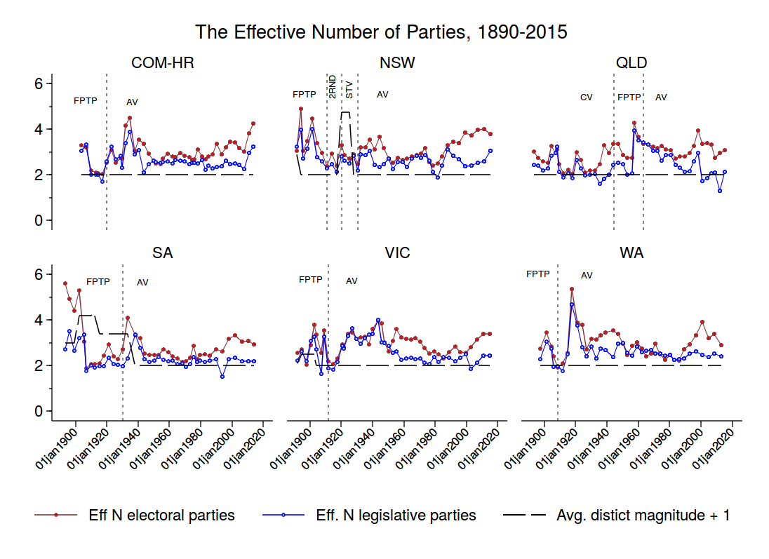
The Canadian data provide a context within which to consider the proportionality of Australia’s AV electoral system. Figure 2 below shows vote shares and seat shares at Australian federal and state elections since 1890. The colour coding in Figure 2 varies by electoral system. So one sees the relationship between votes and seats under not just FPTP and AV but also the Contingent Vote (CV) in Queensland, and STV and 2-round plurality in NSW.

Figure 2. (right-click to enlarge)

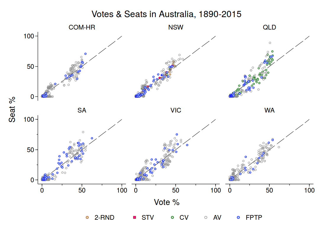
I find three things noteworthy about Figure 2.

1. Australian elections are characterized by disproportionality. Observe that parties that obtain 35-40+% of the vote tend to have seat-shares that fall above the 45° line that marks perfect proportionality.
2. Disproportionality at Australian elections does not appear as severe as it is at Canadian elections. It’s really only in Queensland that the return to votes is visibly non-linear and increasing.
3. It’s not obvious on these data that elections under FPTP were significantly more disproportional than those held under AV.

Of course, these are just my impressions of the visual data; it’s worth exploring the data more systematically. Now, in assessing the votes-seats proportionality of Australian elections we want to:

• account for the fact that some of these elections employed multi-member districts;
• allow the relationship between votes and seats to vary by state; and
• identify the impact on proportionality of shifting from FPTP to AV.

I do all this by: i) controlling for the average district magnitude at election t in state j (M_tj); ii) adding state fixed-effects (STATE_j) to the model and interacting these state fixed-effects with parties’ vote-shares (V%_ijt); and iii) including a dummy variable, AV_jt , that equals 1 when AV is used and 0 when FPTP is used. (Elections that employed other electoral systems are dropped.) The model is

S%_iit = a + d₁M_tj + d₂Y_t + d₃STATE_j + b₁V%_ijt + b₂(V%_ijt * STATE_j) [2]

+ b₃(V%_ijt * AV_jt) + b₄(V%_ijt * STATE_j * AV_jt) + e_ijt.

The quantity of interest here remains the marginal effect of votes on seats, that is, the rate at which vote-shares are translated into seat-shares. The interactions between V%_ijt and STATE_j and AV_jt in Eq 2 allow this rate to vary by state and by electoral system.

Figure 3. (right-click to enlarge)

Figure 3 shows the marginal effect of votes on seats for each state under FPTP and AV. The circles represent the point estimates, and the bars show the 90% confidence intervals surrounding these estimates. So what Figure 3 tells us, for example, is that for every 1% of the vote a party won at elections to the Commonwealth’s House of Representatives (COM-HR) it obtained about 1.08% of the assembly’s seats on average. In other words, Australian federal elections are mildly disproportional. Furthermore, the proximity of the blue and gray dots tells us that the relationship between votes and seats at Commonwealth elections was unaffected by the shift from FPTP to AV.

In the main, the same remarks can be extended to all five mainland states. Only Victorian elections – held under FPTP no less – might, maybe have been proportional. In no state did AV make elections reliably more proportional – though it came close to doing so in Western Australia. Of course, Australian elections were never as disproportional as Canadian federal elections; only elections in Queensland come close – and that probably has a lot more to do with how the Nicklin and Bjelke-Petersen governments malapportioned and gerrymandered electoral districts than the electoral system itself.

To better isolate any causal effect of the electoral system on votes-seats disproportionality, I estimated Eq. 2 again, but with the data limited to just the very last elections held under FPTP and the elections held immediately thereafter on the adoption of AV. This eliminated NSW from the analysis (because NSW experimented with several electoral systems between abandoning FPTP and adopting AV). District magnitudes did not vary within states at these transitional elections, so there was also no need to control for the average district magnitude. The model was then:

S%_iit = a + d₁STATE_j + b₁V%_ijt + b₂(V%_ijt * AV_jt) + e_ijt [2b]

Under this model, the marginal effect of vote-shares on seat-shares under FPTP is given by b₁, whilst under AV it’s given by b₁ + b₂. Estimating Eq. 2 via OLS returned 

b₁ = 1.10 (.04)  b₂ = -.04 (.08)

Adj. R² = .88  RMSE = 8.51

N Obs = 47  N Clusters = 10

Huber-White SE clustered by election in parentheses

Thus the ratio of vote- to seat-shares was 1:1.10 under FPTP and declined to 1:1.06 under AV – BUT this decline is not statistically significant (not by a long-shot). In other words, we can’t rule out that the shift to AV made no difference whatsoever.

Finally, I estimated an Australian analogue to Eq 1b. containing parties’ vote shares and their squared vote shares – but only using data from AV elections:

S%_iit = a + d₁Y_t + d₂STATE_j + b₁V%_ijt + b₂V²%_ijt + e_ijt [3]

Estimating Eq. 3 via OLS yields:

b₁ = .89 (.06)  b₂ = .004 (.0016)

Adj. R² = .88  RMSE = 6.56

N Obs = 1209  N Clusters = 180

Huber-White SE clustered by election in parentheses

These results indicate that AV also generates nonlinear and increasing returns to votes, although not nearly so sharply as in Canada.  The “break-even” point under AV is also lower at 27.5%

Discussion

There’s no reason to expect AV to be any more proportional an electoral system than FPTP. This is because the proportionality of the electoral system is tightly constrained by the number of seats per district, and both AV and FPTP are typically used with single-member districts.

The data from Australian state and federal elections are consistent with this theoretical expectation. Australian elections do not produce the level of disproportionality that is observed in Canadian elections – but this probably has little to do with Australia’s AV electoral system because the adoption of AV in favour of FPTP in Australia had no discernible impact on electoral disproportionality.

What does this mean for electoral reform in Canada? These data suggest that we should not expect the disproportionality of the Canadian electoral system to change appreciably were the Government to choose AV to replace FPTP. Disproportionality systematically favours larger parties over smaller parties, and to that extent the Conservatives should not be particularly apprehensive of a transition to AV. As I observed previously, a shift to AV could position the Conservatives as a right-wing version of the ALP – not often in government, but dominant on their part of the political spectrum. Correspondingly, the NDP and the Greens should not expect an AV electoral system on its own to improve the efficiency with which these two parties translate votes into seats.

In my next post I’ll explore another aspect of AV – it’s volatility.

---

* A big thanks to my colleague, Campbell Sharman for furnishing me with these data.

It’s incredibly difficult to assess the impact of an electoral reform ex ante. The problem is that parties’ and voters’ strategies are endogenous to the electoral system.  This is one reason why the analysis of electoral reform so often has to operate on the basis of first principles. However, given the vagaries of social choice theory (generally no equilibrium for 3+ options in 2+ issue dimensions), there are limits to what we can say on the basis of first principles. For this reason, it’s still useful (and interesting) to look at data to learn about the impact of electoral reform.

The Spaniel is on record as preferring a “ranked ballot” electoral system – or the “Alternative Vote” (AV) as the system is known in Australia, where it has long been used at federal and state elections.[1]  With their majority, the Liberals can impose an AV on the country – and, as I have argued previously, they have strong incentives to do so. Theoretically, AV works to the advantage of large, centrist parties like the Liberals. Correspondingly, it (theoretically) works to the disadvantage of both smaller parties and identifiably left- or right-wing parties; the former are disadvantaged by AV’s use of single-member districts; the latter, by the fact that they are less likely to be the second-preference of many voters.

Given that, it is interesting to look at how AV has worked out Australia, how the transition from FPTP to AV in Australia altered the effective number of parties that contested elections and won seats, the proportionality between votes & seats, the support for third-parties, and the level of electoral volatility. (Keep in mind that electoral reform was itself often undertaken by incumbent government’s in response to a threatening change in the party system, e.g., a growing Labor party.)

The Australian experience with AV is quite unique; I know of no other major country that has had such long experience with AV.  But that makes it problematic to draw inferences about how AV might affect Canadian politics: we can’t know which aspects of Australian electoral and party competition are due to the inherent dynamics of AV and which are due to Australia being, well, Australia.  To get around this (but, to be honest, only part way around this), I examine elections in Australia’s five mainland states as well as in the Commonwealth.[2]  To the extent that trends are common across all 5 states and the Commonwealth, we can assume that that’s due to the (common) electoral system and not the peculiarities of the state.

The Australian state data are especially useful because, like the Commonwealth, the five mainland states used FPTP before adopting AV. This allows one to assess the impact of transitioning from FPTP to AV within each state.  Now, the transition was not always direct as Table 1 below shows: NSW experimented with a two-round plurality system (of the sort used for elections to the French National Assembly), STV, and the Contingent Vote before adopting AV; Queensland only adopted AV in 1963.[3]  In addition, FPTP was not always employed with single-member districts. South Australia applied both the plurality rule and the alternative vote in 2- and 3-seat districts.

 

Table 1.  Electoral Systems used in Australia, 1890-2015

	C-W	NSW	QLD	SA	VIC	WA
FPTP	1903-17	1891-1907	1941-60	1893-1927	1892-1908	1890-1905
2-RND		1910-17
STV		1920-25
CV		1927	1893-1941
AV	1919-		1963-	1930-	1911-	1908-

The Effective Number of Parties

One of the first things a political scientist likes to know about a country is how many parties contest elections and win seats.  The longstanding notion is that the number of parties is closely related to political stability, the potential for polarization, and the capacity of electoral politics to represent diverse interests. Now, not every party counts as interesting or relevant; for example, we probably want to discount fringe parties that obtain .5% of the vote — but arbitrarily ignoring some parties (which ones?) is problematic.  Consequently, political scientists tend to focus on the effective number of parties (Laakso & Taagepera 1979).  We either count the effective number of electoral parties (i.e., the number that contest elections) and/or the effective number of legislative parties (i.e., the number that win parliamentary seats).  We obtain the effective number of electoral parties by constructing a Herfindahl-Hirschman Index (HHI) of parties’ vote shares, with vote shares expressed as proportions.  Similarly, we obtain the effective number of legislative parties by constructing a HHI of parties’ seat shares, with seat shares expressed as proportions.  (The difference between the two statistics can be informative.  For example, we often see large deficits in the number of parties that contest elections and win seats in transitional democracies where expectations about parties’ competitiveness have not yet congealed.)

The Effective Number of Parties in Australia, 1890-2015

Figure 1 shows the effective number of electoral and legislative parties in the Australian Commonwealth and the five mainland states over time. These statistics provide a rough means to track the relationship between the electoral system and the party system. For example, we can use the data in Figure 1 to assess if changes to the electoral system precede sharp changes in in the number of parties that contest elections or win seats.

 

(Click on the figure to enlarge it)

From a theoretical perspective, one would not expect a shift from FPTP to AV to have a big impact on the effective number of parties. This is because both systems tend to be used in conjunction with single-member districts (i.e., districts magnitude = 1), and theory (Cox 1997) predicts M + 1 effective parties to contest elections. (And, because parties are unlikely to persist in contesting elections unless win at least some seats, to secure legislative representation, we might also predict M+1 legislative parties). The prediction is a weak one, however, because Cox’s M+1 rule operates at the district-level – and different sets of M + 1 parties could present themselves in different districts. Still, the dashed line in each panel of Figure 1 shows this M+1 threshold for each state.

Between 1940 and 1980, South Australia’s party system closely adhered to this theoretical prediction, with just 2.5 effective electoral parties and 2.25 effective legislative parties. However, the main message of Figure 1 is that the effective number of electoral and legislative parties can and does wander from this M+1 equilibrium. Observe, for example, the growth in the number of electoral parties in the post-1980 period at both state and federal levels. Plainly this post-1980 increase in electoral parties is not due to the main features of the electoral system because by this point in time all mainland state and federal elections in Australia were held under AV.

In addition, the effective number of electoral and legislative parties was pretty much the same under FPTP and AV controlling for differences in district magnitude. The effective number of electoral parties in each state and federally averaged about 3 (i.e., M + 2), and the effective number of legislative parties in averaged about 2.5 — and did so under both FPTP and AV.

Nor is there any evidence that changing the electoral formula from plurality to AV leads to changes in the effective number of electoral or legislative parties. Indeed, the evidence on this front is far more consistent with Cox’s view that it is mainly the district magnitude that shapes party competition. To show this, I ran regressions of year-to-year changes (i.e., first-differences) in the effective number of electoral (ΔENEP) and legislative parties (ΔENLP) on contemporaneous and lagged changes in the electoral formula (ΔF, ΔF_t-1) and district magnitude (ΔM, ΔM_t-1):

ΔENEP_st = a + b₁ΔF_st + b₂ΔF_st-1 + b₃ΔM_st + b₄ΔM_st-1 + u_st (1)

ΔENLP_st = a + d₁ΔF_st + d₂ΔF_st-1 + d₃ΔM_st + d₄ΔM_st-1 + e_st (2)

The results (below) indicate that 1) an increase in the district magnitude in year t increases the number of electoral parties by .34 in t and the number of legislative parties by .21 in t+1.[4]

Table 2. OLS Model of Changes in the Effective Number of Electoral and Legislative parties

The Effective Number of Parties in Australia, 1890-2015

	ΔENEPst	ΔENLPst
ΔFst	–.29 (.15)	–.14 (.17)
ΔFst-1	.23 (.23)	–.03 (.08)
ΔMst	.34*** (.07)	.09 (.13)
ΔMst-1	–.10 (.26)	.21*** (.05)
Constant	–.005 (.01)	–.01 (.006)
N Obs	239	239
R2 = .04	.04	.02

Robust SE clustered by state in parentheses

Conclusion

What these data suggest is that the introduction of AV in Canada is unlikely to generate major changes in the effective number of parties that contest elections or win seats. Canadian federal elections from 1949-2015 have been contested by 3.3 effective electoral parties, and produced an average of 2.5 electoral parties (not far off the Australian figures). The adoption of AV can be expected to leave these statistics intact precisely because such a reform would leave the district magnitude intact. This does not, of course, rule out changes in the identity of parties that contest elections or win seats or the possibility of major shifts in vote- or seat-shares between parties (because the effective number of parties remains the same whether the Liberals gain 35% of the vote, and the NDP, 15%, or the converse.)

In the next post, I’ll consider if/how the transition from FPTP to AV in Australia altered votes-seats proportionality.

---

 

[1]  Under AV, voters (typically in single-member districts) rank their preferred candidates from 1-N. If any candidate secures 50+% of voters’ first-preferences, s/he is declared elected. If not, the lowest ranked candidate is eliminated and ballots cast for the eliminated candidate are distributed to the remaining candidates according to second-preferences. If any candidate secures 50+% of voters’ first- and second-preferences, s/he is declared elected. If not, the lowest ranked candidate is again eliminated and ballots redistributed, etc.

[2] Many thanks to my colleague, Campbell Sharman, for furnishing me all these data on Australian elections.

[3]  The contingent vote (CV) is a hybrid between FPTP and AV: Under CV, the voter lists up to two preferences on their ballot, one for the most-preferred candidate and a second-preference for another candidate. If there is no majority-winner on first-preferences, then all candidates but the top-two are eliminated, and ballots cast for those candidates are redistributed according to second preferences. The winner is then the candidate with the plurality of first- and second-preferences.

[4]  Using first-differences obviates the need to include state fixed-effects. Now, the model does restrict the coefficients to be the same across states, but there’s not really enough variation to allow for the coefficients to vary by state.  Also, it’s clear that changes in formula include shifts from say, STV to CV, as in NSW; they are not just confined to transitions from FPTP to AV. But the results are largely unaffected by, say, dropping NSW from the model.