Tag Archives: geography

Applications of GIS in Health Geography

Today’s lecture focused on the major applications of GIS in health geography:

  1. Environmental hazards
  2. Modelling health services
  3. Identifying health inequalities
  4. Spatial epidemiology (the focus of today’s lecture)

This lecture covered multiple definitions of health and disease, discussed how location matters. The focus was on spatial epidemiology, or “the study of the distribution and determinants of health and disease-related states in populations, and the application of this study to control health problems” (slides). To study disease, we need measures of its occurrence such as counts, prevalence, incidence, and mortality. It is also useful to use a small area of analysis in order to explore the existence of a relationship between variables (such as environment and health). We can control for other relevant factors using regression.

It is important to recognize that a small scale may present issues with your analysis:

  1. Spatial misalignment
  • This can become an issue especially when you are using data from different institutions. Misalignments may not have posed an issue at smaller scales, but a large scale (small area) analysis makes these spatial discrepancies obvious and problematic.

2. Uncertainty

  • How often is population data collected? Are we confident about it’s quality? Is it accessible/available to use? How do you measure a population’s exposure to an environmental variable? Are environmental impacts distinguishable from lifestyle or socioeconomic impacts on health?

A take-home point was that doing analysis of disease rates or counts in small areas often involves a trade off. How do we balance statistical stability of the estimates and geographic precision?

What is Health Geography?

It shouldn’t come as a surprise that health and geography are intrinsically linked. The places we spend time in influence our access and exposure to determinants of health – pollutants, disease, food and nutrients, health services, and more.

The lecture included examples such as the relationships between climate, elevation & distribution of malaria, as well as the connections between exposure to fast food restaurants and childhood obesity rates. These were definitely useful to generate potential topics for the class project.. (perhaps the geographical distribution of radon and incidences of respiratory cancer?)

We compared definitions and perspectives of medical and health geography, epidemiology and environmental justice. Health geography combines qualitative and quantitative methods, and considers the special role of “place”  in determining health. A geographical perspective is useful because we, as geographers, tend to focus on the relationship between people, place, and “space.” In this vein, geographers emphasize the importance of considering local contexts (including societal factors).  A regional/national/international scale of study can be useful, but it is not sufficient. This unique contribution to health geography research can be observed in methodological developments including multi-level statistical models, cluster analysis and geographically weighted regression.

Why is geography important?

Lecture 01.10.18

So… geography. Why is it so important?

Just like I mentioned in my last post, geography is a natural element of any and all analysis. Today’s lecture delved further into this idea to consider various issues arising from any study that uses geographic data, including:

  • the modifiable areal unit problem (MAUP)
  • the scale, grain and extent of a study
  • the nature of the boundaries of a study area
  • spatial dependence / heterogeneity.

Continue reading

Final Project: Assessing Vancouver’s Livability for Seniors

This project aimed to determine which neighbourhoods of Metro Vancouver are best suited for senior citizens. Our analysis was based on the assumptions that seniors would prefer areas of low housing costs, low crime rates, and that have senior-targeted amenities within an accessible walking distance.

Click here to see the Final Project Report!

Our team met at least once every week to construct the maps together. We typically had one member operating ArcMap, with another looking over their shoulder offering guidance and looking up instructions and online help. Another group member would be recording the steps taken in order to assemble a flow chart at the end of the project process. The final report was divided into sections amongst the group to be written up, but was edited together.

According to our analysis, the three best neighbourhoods for senior citizens in Metro Vancouver are:

  1.  Renfrew Collingwood

  2. Strathcona

  3. Marpole (eastern portion)

The project helped us be to become more familiar with the spatial join tool in particular. This skill allowed us to normalize data points, such as break and enters, over neighbourhoods. This suited our goal of comparing Vancouver neighbourhood crime rates and other factors.

We also became more comfortable with retrieving data from external sources. Census data was simple to find. We had originally planned to include grocery stores in our amenities analysis, but had significant difficulty in locating data. We acknowledge that this would be a good thing to include in future analysis of liveability in our report.

Group projects, particularly with GIS, face a multitude of challenges. There are several people working on the same set of maps which means that communication is key. We found that creating a Google doc to record notes, steps taken, and thoughts/ideas throughout the project process allowed all group members to stay on the same page. It was handy for both facilitating good group communication and later for creating the flow charts. It also made data management much more simple, because names of files were recorded with a description.

We also created a Facebook group for efficient communication. This was what we used to schedule group meetings and send documents/maps.

LAB 5: Environmental Assessment

In this lab, we performed an environmental assessment of the Garibaldi at Squamish ski resort. I was tasked with assessing the project as a (pretend) natural resource planner obtained by the British Columbia Snowmobile Federation (BCSF).

When working on environmental projects, you sometimes become involved in proposals that you do not ethically believe in. Although my conclusion as an analyst hired by the BCSF argues that the project should go ahead, my personal opinion is against the development of this project. Considering the project will likely be negatively affected by climate change in the not-so-far future, the potential environmental damage caused by this development is not ‘worth’ the economic gains.

Click here to see my map of the project area!

Click here to see my 3D Hillshade Map!

Here is my memo created following the environmental assessment:

THE PROPOSED PROJECT

The Garibaldi at Squamish project is a proposed year-round destination mountain resort between Squamish and Whistler on Highway 99. Proposed by Northland Properties and Aquilini Investment Group of Vancouver, the project includes 124 ski trails and 21 lifts, resort accommodation and commercial developments. It is located on Brohm Ridge; 80 km north of Vancouver, 15 km north of Squamish, and 45 km south of Whistler. Despite being very controversial due to concerns over the economic viability, climatological implications, and environmental impact on vegetation and fish and wildlife habitat, the project was tentatively approved in January 2016 provided it meet 40 conditions.

My involvement in it:

I am a natural resource planner retained by the British Columbia Snowmobile Federation (BCSF). The BCSF is currently in opposition to the proposed project, but wish to evaluate whether there is sufficient evidence to continue to oppose the project, or whether these aforementioned concerns can be addressed. I will examine the Environmental Assessment’s recommendations and the Resort Municipality of Whistler’s criticism (of climate limiting viability of skiing) to accomplish this task.

The analysis:

This analysis aims to ultimately determine whether the proposed Garibaldi at Squamish project is economically viable. If the proposed project is a ‘good’ fit for the area, it may be successful at drawing in tourism and increasing local business for the BCSF — and thus should be supported by the BCSF. Using data acquired from DataBC and the BC Government, I considered environmental protection areas, road accessibility, and the future of snow in the park area in my analysis. A ‘good’ fit would ultimately be if few new roads are required, there is little encroachment on environmentally protected areas, and that snow supply is sufficient and reliable in the project area.

Future of snow:

The Resort Municipality of Whistler argued that reliable skiing would be limited on the lower 555m of vertical in the project area. In my analysis, I reclassified areas of the proposed project area that were below 600 metres using digital elevation model data – assuming that climate change would limit snow in these areas.

Environmental protection areas:
The environmental assessment was simplified; data was filtered to consider the ungulate winter range, old growth management areas, riparian habitat, and endangered/threatened ecosystems. All data was clipped to focus only within the proposed project boundaries. Riparian habitat determined necessary to protect was set within a 100m distance of lower elevation streams (below 600m elevation) and 50 metres of streams above 600m elevation with a simple buffer proximity analysis.

RESULTS

Environmental Protection:

Of the proposed project area:

  • 6.8% contains old growth forest
  • 7.9% contains Mule Deer and/or Mountain Goat habitat
  • 24.8% contains red-listed species (6 endangered/threatened species total)
  • 26.3% contains riparian habitat zones
  • The total project area that will directly impact old growth forest, ungulate habitat, red-listed ecosystems and fish is 52.7%.


Future of Snow:

38.6% of the proposed project area is below 600m, and these areas are thus predicted to be inadequate for reliable skiing.

RECCOMENDATIONS

Despite large portions of the proposed project area being occupied by areas in need of environmental projection and/or having limited snow supply, it is important to consider that most of these areas appear to occupy much of the same space. As can be seen on the maps, red-listed species overwhelmingly reside in lower elevation areas, for instance. There remains a large portion of the project area that could be operated upon without concerns of snow supply, and the lesser environmental concerns there might be mitigated.

The two greatest environmental concerns to project development are encroachment on red-listed species habitat and riparian habitat. Large portions of both riparian habitat zones and red-listed species habitat are both found in the areas below 600m elevation areas that are predicted to be unusable for skiing anyways. These important habitats can be mostly protected if developers simply avoid these low elevation areas. Threats to riparian habitat in higher elevation areas could be mitigated by keeping new road and other infrastructure development outside the 50m buffer areas used in this analysis.

Ultimately, there is still a large portion of the proposed project area that could prove to be economically viable. Most of the proposed project area is still above 600 meters and will most likely have reliable skiing into the future. It is in the best interests of the BCSF to support the Garibaldi at Squamish project.

LAB 1-3 Accomplishment Statements

Accomplishments so far?

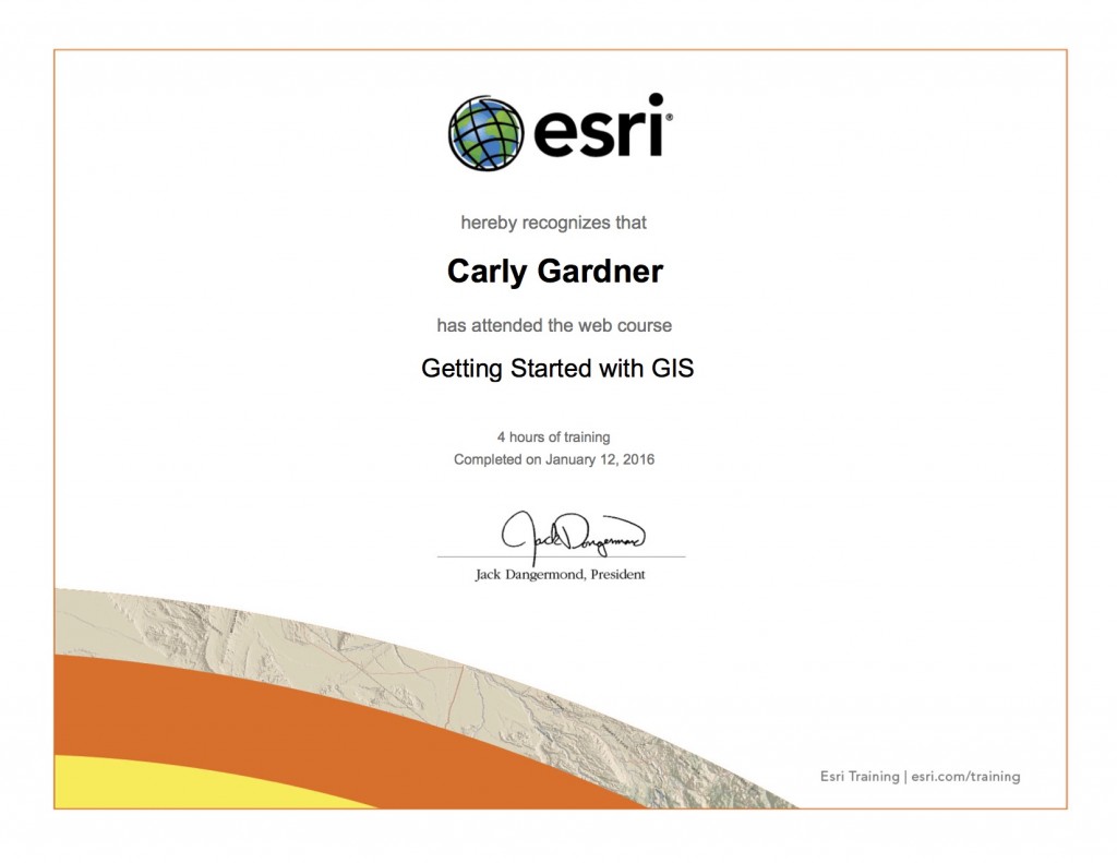
Lab 1: Completed an introductory ArcGIS course offered by ESRI and reviewed examples of GIS applications to gain foundational knowledge for future GIS projects.

Lab 2: Gained practical working knowledge of coordinate systems and projections and how to fix misaligned or improperly referenced spatial data for geographic analysis.

Lab 3: Used spatial and tabular data sets to perform geographic analysis of Vancouver’s tsunami risk, generated a  corresponding map and useful statistics.

LAB 4 Part 2: Housing Affordability

In this part of the lab, we created maps of the affordability in both Vancouver and Ottawa. We used manual breaks as our classification method, setting the same break values in both maps. This allowed us to compare the housing affordability of both two cities to each other!

Click here to see my Housing Affordability maps!

Affordability is considers median housing cost normalized by income. So areas that have high housing cost and high incomes are considered more affordable than areas with high housing costs and low incomes. This is a better indicator of housing affordability than housing costs alone, because it is a more appropriate indicator of liveability. High housing costs become a more important issue when those living there do not have high enough incomes to afford it. For instance, housing costs in New York City are extremely high but its residents typically have high incomes. In contrast, Vancouver housing costs are high but residents have lower incomes. Vancouver is less affordable despite having cheaper housing costs than New York City.

The housing affordability rating categories used in my maps are:

  • no data
  • affordable (3.0 and Under)
  • moderately unaffordable (3.1 – 4.0)
  • seriously unaffordable (4.1 – 5.0)
  • severely unaffordable (5.1 and Over)

These categories were determined by the 12th Annual Demographia International Housing Affordability Survey: 2016 (www.demographia.com/dhi.pdf).  For the purposes of my map, I believe these categories are to be trusted.

Affordability is a good indicator of a city’s ‘liveability’, but should not be the sole indicator used. There are many other factors that influence ‘liveability’, including business conditions, environmental conditions, crime, transport networks etc.

LAB 4 Part 1: Quantitative Data Classification

In Lab 4, we accessed Canadian census data to map the affordability of Ottawa and Vancouver.  The objectives were to familiarize with the various methods of classifying data and to explore their potential ethical implications.

Click here to see my Data Classification Maps!

Part of the lab instructed students to pretend we were journalists hired to report on the affordability and liveability of Vancouver. Which data classification method would a journalist use to display affordability of Vancouver? As a journalist, I would likely choose manual breaks because it would allow me to compare a map of Vancouver’s housing costs to maps of other cities’ (that have the same breaks). This could illustrate that Vancouver’s housing is extremely unaffordable, even when compared to other areas (or visa versa) – the potential for a story.

However, if I were a real estate agent preparing a presentation  for prospective home buyers near UBC, I would use standard deviation as my data classification method.  UBC property appears to be relatively inexpensive with this classification. Because it is located next to areas that appear very pricey, potential buyers might view purchasing UBC property as an opportunity for investment (UBC might be predicted to follow the rising housing values of the surrounding area).

It is important to note that the different methods of classification may influence the interpretation of data on maps, and that there might be ethical implications. Is if fair to choose classifications that overemphasize ‘affordable’ and ‘unaffordable’ areas of Vancouver? That might mislead potential buyers. What if the division of your data classes is confusing to viewers?

LAB 1: Intro to GIS

ESRI certificate ESRI certificatejpeg

In this lab, I completed an online tutorial of ESRI’s GIS software. It provided me with an introduction to the basics of ArcGIS, including how to:

  • display map features
  • add data to a map
  • manipulate data tables
  • create a map (layout)
  • save a map and associated data files

I also considered issues of data integrity and ethical implications for GIS mapping.