Author Archives: carly gardner

Here’s the abstract of our final project, also available for viewing at blogs.ubc.ca/mappinglungcancer.

TITLE

Lung Cancer Mortality in the Eastern United States: A Geographical Perspective

AUTHORS

Carly Gardner and Evan Morrow

OBJECTIVES

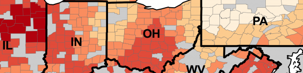
We examined geographic patterns of lung cancer mortality in the eastern United States. We focused on counties in order to reveal smaller scale variance in environmental and socioeconomic factors associated with lung cancer.

METHODS

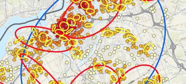
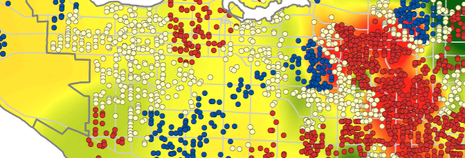
We used ESRI’s ArcMap to generate hot spot maps and to conduct ordinary least squares (OLS) and geographically-weighted regression (GWR). County-level socioeconomic data was provided by the US Census Bureau (1999, 2000). Lung cancer mortality rates were collected from the Centers for Disease Control and Prevention WONDER Online Database (1999-2003). County-level smoking prevalence in 1999 was provided by Dwyer-Lindgren et al. (2014).

RESULTS

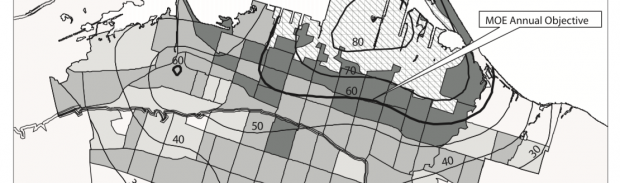
The GWR had a higher adjusted r-squared value (0.62) than in OLS Models 1 (0.48) and 2 (0.54). Highest local r-squared values were present on the western side of the region, particularly in northern Georgia, northeastern Alabama, and Tennessee (0.64 – 0.72). The proportion of rented homes, proportion of non-white population, median income and radon risk were each significantly associated with county-level lung cancer mortality rates, relationships that were spatially non-stationary across the eastern United States.

CONCLUSION

The results of our analysis indicate that, aside from smoking prevalence, there are numerous statistically significant variables that are associated with lung cancer mortality. Our analysis provides evidence that the associations between lung cancer mortality and numerous socioeconomic and environmental parameters vary across space. It calls for local context-specific efforts to address lung cancer mortality in the eastern United States.

Class was cancelled on Friday, so the geography students didn’t have to present the assignments we had created. But, we did get to listen to the presentations from the GEM students!  This week’s topic was crime and geography.

One particularly interesting (but rather depressing) presentation was called A Geospatial Analysis of Suicidal Bridge Jumping in the Metro Vancouver Regional District from 2006 to 2014. Suicide was decriminalized in 1972, but it is still relevant to this week’s topic.

The study by Lam, Kinney and Bell was interested in how suicide victims navigate their environment to choose a preferential place for committing suicide. Using the network analyst tool in ArcGIS, the authors found that most victims are willing to travel further distances to jump from more iconic and symbolic locations, such as Lionsgate Bridge (the most popular location to jump in Metro Vancouver). These victims were classified as ‘travel jumpers,’ in contrast to the much smaller number of ‘convenience jumpers’ (those who jump from locations that are close to their homes).

The paper Evan and I covered was called Space-Time Dynamics of Crime in Transport Nodes by V. Ceccato and A.C. Uittenbogaard. The objective of this study was to assess space-time variations of crime at underground stations in Stockholm, Sweden. They began with two hypotheses:

1. Crime in underground stations reflects rhythmic variations of human activities (hourly, daily, weekly and seasonally).
2. The specific vulnerability to crime of a transport node varies over time and space.

The analysis used ANOVA and Sheffe’s test and OLS regression models to check for crime variations over time. The paper outlined many of their results in great detail. Some of their findings were that:

• peaks of crime in late afternoons and evenings, when most people are on the move. Therefore there is a greater risk of victimization.
• most crimes late in the evening and night were violent.
• vandalism takes place more often during late evenings.
• thefts occur most often in the afternoon and early evening.

All in all, we awarded this paper a 7/10. The methods and results were meticulously outlined (but almost too much – it was quite overwhelming to read). The OLS model was properly specified, and variables with potential multicollinearity were removed. Although acknowledged, there was potential for subjectivity when quantifying data such as the station atmosphere and environment. These were values that were rated on a scale according to the personal impressions of the two researchers. They also could have gone further with data visualization – it was a lost opportunity!

This week was another round of presentations! As the title of this post implies, the topic of this assignment was health geography and GIS.

My favourite presentation was regarding the research paper: Using geographically weighted regression for environmental justice and analysis: Cumulative cancer risks from air toxics in Florida. This study focused on two research questions:

1. Are cumulative lifetime cancer risks from ambient exposure to multiple sources of hazardous air pollutants distributed inequitably with respect to race/ethnicity and socioeconomic status across Florida?
2. How does the direction and significance of statistical relationships between cumulative lifetime cancer risk and race/ethnicity or socioeconomic status vary across the state of Florida?

The paper used both Ordinary Least Squares and Geographically Weighted Regression in their analyses. The found a significant positive relationship between the proportion of Black, Hispanic and Asian residents and cancer risk, and a significant negative relationship between population density, poverty and cancer risk.

This presentation has gotten me thinking about ideas for the final project! It might be interesting to explore other geographic patterns of health…

—-

This week was Evan’s turn to present on our behalf. The research paper we chose was A GIS-environmental justice analysis of particulate air pollution in Hamilton, Canada by Jerret at al., 2001.

The two primary objectives of the study were to analyze the relationship between total suspended particulate (TSP) exposure and socioeconomic variables such as income, unemployment and housing value with an environmental justice/equity framework; and to look at how sensitive the relationship between air pollution and socioeconomic variables is to specification of exposure estimates or statistical models.

To do this, they created two different exposure maps (chronic and extreme) which were input into OLS and simultaneous autoregressive (SAR) analysis with socioeconomic data (income, dwelling value, unemployment rate etc). They found that there was a difference in significant variables depending on the model used. For instance, dwelling value and low income were significant in OLS models, but in SAR the low income variable was replaced by unemployment. In both models, dwelling value was the most significant independent variable. They also found that highest exposure zones have a twofold increase in total suspended particulate concentrations and a more than twentyfold difference in probability of exposure to extreme events than lowest exposure zones.

All in all, we gave this paper an 8/10 because their findings generally aligned with other research, steps were taken to properly specify the models, and sources of error and uncertainty were acknowledged. Their maps are simple and effective. Our primary complaint was that the models are slightly outdated now.