As mentioned in my previous post, Geographically-Weighted Regression (GWR) is an extremely effective regression model for spatial analysis, especially when there may be regional variance in the relationships between independent and dependent variables. GWR allows us to explore the local relations amongst a set of variables, and to examine the results spatially using ArcGIS; it can even produce raster coefficient surfaces which allow us to see any regional variation in the relationships of the parameters! We can see if the variables and residuals of the model are spatially dependent or spatially autocorrelated.
In this lab, we explored the relation between a child’s social skills and various socio-demographic variables related to the child and to their neighbourhood. First, we began with an explanatory regression analysis to determine which variables (average income, gender, and language ability) had the strongest relationship with children’s social scores.
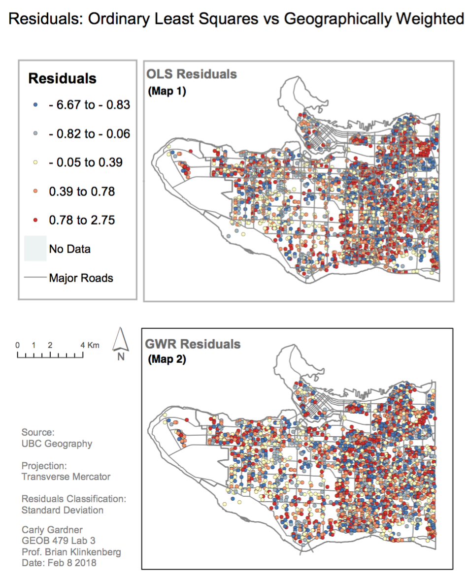
This was followed by an Ordinary Least Squares (OLS) analysis to examine the correlation between these selected variables across Vancouver. However, a basic linear regression analysis like OLS assumes that the relationships between variables remains constant over space. Recognizing that there is likely some spatial autocorrelation and variance across the region, we also conducted a GWR. In a comparison of OLS and GWR residuals, it is clear that there are differences between them, suggesting that regional influences on social scores vary across space, and that there is more pronounced or significant variability in the relationships between social scores and its explanatory variables in areas of East Vancouver.
When overlaid by the local R-squared results generated by the GWR regression, there appear to be certain neighbourhoods of Vancouver which display a strong correlation with social scores (Map 3). These neighbourhoods were generated by a grouping analysis that combined regions of similar traits.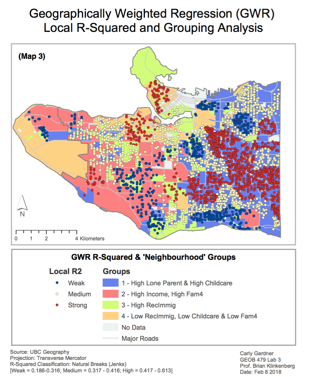
When working with socio-economic variables and real people, the amount of ‘explanation’ a statistical model can produce is quite limited. It should be noted that strong R- squared values in this analysis range from 0.416 to 0.613.
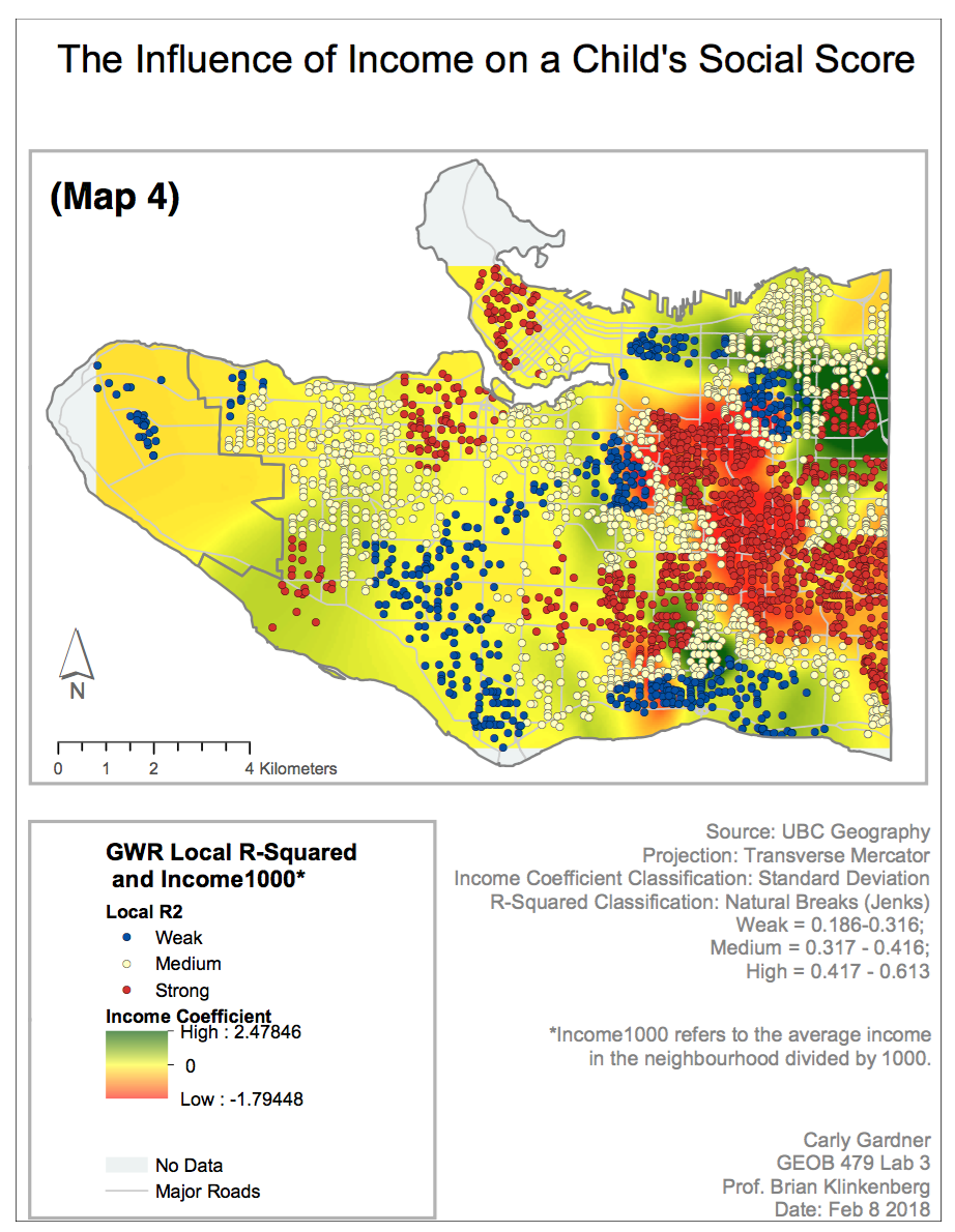 In areas like Kensington-Cedar Cottage, where there is statistical significance suggested by strong R-squared values, we can see particularly strong correlation between social scores and language ability (positive), and between social scores and income (negative). This is consistent across areas like the Kensington-Cedar Cottage neighbourhood.
